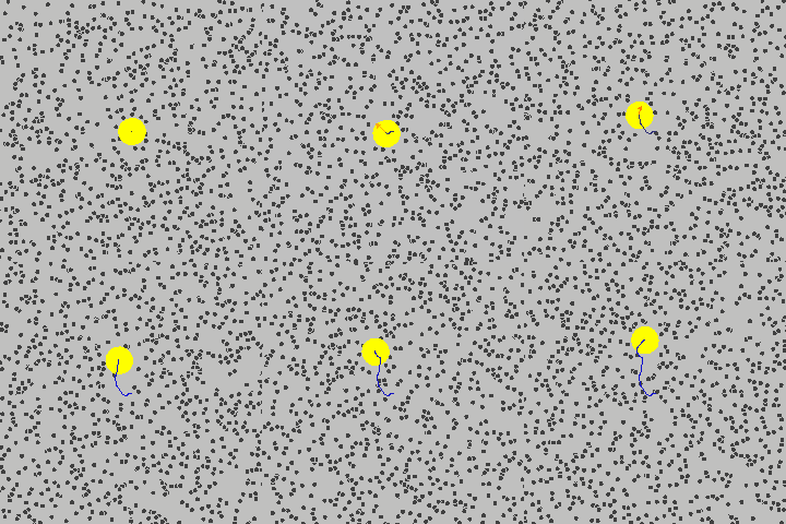
source: https://en.wikipedia.org/wiki/Brownian_motion
DSI Studio is an open-source diffusion MRI analysis tool
that maps brain connections and correlates findings with neuropsychological disorders.
It is a collective implementation of several methods, including DTI, QBI, DSI, generalized
q-sampling imaging, q-space diffeomorphic reconstruction, diffusion MRI connectometry, and
generalized deterministic fiber tracking.

source: https://en.wikipedia.org/wiki/Brownian_motion

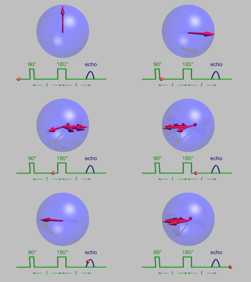
source:http://dsi-studio.labsolver.org/course/diffusion-mri-signals
The effect of diffusion on the MR signal was mentioned by Hahn in 1950.
The diffusion coefficient can thus be measured by acquiring diffusion signals with difference gradient strength |g|.

source: Sosnovik, D. E., Wang, R., Dai, G., Reese, T. G., & Wedeen, V. J. (2009). Diffusion MR tractography of the heart. Journal of Cardiovascular Magnetic Resonance, 11(1), 1-15. link
whereas S is the DWI signal. S0 is the DWI signals without diffusion weighting (also known as the b0 signal)
The apparent diffusion coefficient, as explained by its naming, is the diffusion coefficient “appearing” from the observation of a heterogeneous environment (e.g. biological tissues).

Figure: Jellison, Brian J., et al. "Diffusion tensor imaging of cerebral white matter: a pictorial review of physics, fiber tract anatomy, and tumor imaging patterns."American Journal of Neuroradiology 25.3 (2004): 356-369.

There are numerous variants of the deterministic fiber tracking, and they can be further classified by the following feature.
There are parameters affecting tracking results.
The following is a list of the region types.
A diffusion tensor can provide fractional anisotropy (FA), axial diffusivity (AD), radial diffusivity (RD), and mean diffusivity (MD).

DICOM Format, including image acquired by SIEMENS TIM, SIEMENS Trio, GE SIGNA HDx, and Philips 4D DICOM.
Analyze format, Nifti format, 3D volume or 4D volume (diffusion space as the highest dimension order)
Bruker 2dseq files
Varian and Agilent FDF files

Before using the DICOM files, I would recommend rename them using [Tool: Batch processing][Rename DICOM files] and select all the DICOM files that are ready to be renamed, and then the file will be moved into its related folders. You may also use [Rename DICPOM in subfolders] to assign a root folder containing all DICOM files to be sorted. DSI Studio will rename DICOM files and place them in different folders according to their pulse sequences (see figure to the right).
Check b vector or add b vector

It is recommend that the SRC files are examined by a quality control procedure to ensure its integrity and quality. To do this, use [Tools: Batch Processing][SRC Files Quality Control] and select the folder that contains SRC files (DSI Studio will search for all SRC files in the subdirectories).
first thing to check is the consistency of image dimension, resolution, DWI count, shell count. It is likely that certain scans are incomplete, and the total DWI count will be different (see subject 102008 in the example.
second thing to check is the “neighboring DWI correlation”. “Neighboring DWI correlation” calculates the correlation coefficient of low-b DWI volumes that have similar gradient direction. Higher correlation indicates good quality. The value will decrease if there is a prominent eddy current artifact, head motion, or any head coil issues that may impact the diffusion signals. It is recommended to use an outlier checking function (e.g. 3 median absolute deviation) to spot problematic data or simply sort this values and inspect subjects with low correlations to see if there is any quality issue. The example on the top identifies a dataset with a neighboring DWI correlation of only 0.892282, which is substantially lower than the other. Another dataset 102008 has a different b-table, which cannot be used together with the others.
If a dataset has a very low niehgboring DWI correlation, you will need to examine the raw DWI images. To inspect individual SRC file, open it in STEP2 reconstruction and switch to the first tab that shows the raw images. You may scroll through all DWI to see if there is prominent movement, signal dropout, or any other issues. A good DWI data set should have normal signals intensity decrease as b-value goes up. Any abnormal signals drop indicates possible problem.
Open DSI Studio and press the “step 2: reconstruction” button in the main project window to select the .src file. DSI Studio will present a reconstruction window as shown in the figure to the right.
STEP1: Setup a Mask

Recommendation steps include thresholding, smoothing, and defragment.
STEP2: Select a Reconstruction Method

The meaning of the diffusion indices can be found here: https://sites.google.com/a/labsolver.org/dsi-studio/course/diffusion-mri-connectomics?pli=1#TOC-Introduction-to-diffusion-Indices.
The steps to create a tractography are as follows
Step1. Assign Regions
![]()
DSI Studio provides a handy list of atlases that can be added to the region list. Users can add a known anatomy by click on the “atlas” button in the “Region List” window. The atlas is mapped to subject space by nonlinear registration between the anisotropy map and the atlas included in the DSI Studio package.
The atlases include the following:
There are several region types available to control fiber tracking
Step2. Setup Tracking Parameters
![]()
Step3. Perform fiber tracking and save tract coordinates
Use “whole brain seeding” always. DSI Studio will assign whole brain seeding if you do not specify a seed region. Please note that the tracking algorithm starts from the seeding point and track in two directions until it reaches the ending points. In most of the cases, the seeding point is not the end points of the trajectory.
To track trajectories connecting between two brain regions, place two “end” regions, one on each of them. DSI Studio will find the trajectories that end in these two regions.
An “end” region is more restrictive than a “roi”. A “roi” allows tracks to pass through, whereas the end region requires that the trajectories end in them. If you cannot find connections using two end regions, try setting them as roi.
To force track to terminate if the anisotropy threshold is “greater” than a value. First, set up the threshold to the designated value and place whole brain seed by [Regions][Whole Brain Seeding]. In the region list window, change the region type from “Seed” to “Terminative”. This will enforce a termination if tracks enter the region. Adjust the threshold to a lower value to initiate fiber tracking.
Shortcuts and Controls
In the ROI window:
Key “Q” and “A”: move sagittal slide
Key “W” and “S”: move coronal slide
Key “E” and “D”: move axial slide
Key “Z”: switch to sagittal view
Key “X”: switch to coronal view
Key “C”: switch to axial view
Double click: move slices to the pointed location
In the 3D window
Mouse left button: press and rotate the object
Mouse right button: press and change the zoom scale
Mouse mid button: press and move the object (you may also use direction keys to move the object)
Ctrl+A: move ROI or slides in the 3D window (drag)
rack editing
The following four shortcuts are for tract editing. To edit the tracts, 1) hit the shortcut 2) press left mouse button 3) drag the cursor 4) release the mouse button. If the track selection further considers the income angle, use right mouse button instead. (please refer to here for details)
Ctrl+S: select tracts in the 3D window
Ctrl+D: delete tracts in the 3D window
Ctrl+P: delete tracts in the 3D window
Ctrl+X: cut tracts in the 3D window (click-drag-release)(cannot undo)
Ctrl+T: trim tracts
Ctrl+Z: undo select and delete
Ctrl+Y: redo select and delete
STEP 1: Reconstruction
STEP 2: Whole brain fiber tracking
STEP 3: Brain parcellations
STEP 4: Connectivity matrix
STEP 5: Network analysis

In the connectivity matrix dialog, switch to the “network measures” tab (as shown in the figure) to view the results of graph theoretical analysis.
Graph theoretical analysis views brain connections as a graph and applied graph-based measures to analysis it. A graph is defined as a set of nodes or vertices and the edges or lines between them. Its topology can be quantitatively described by a wide variety of measures, including network characteristic path length, clustering coefficient, global efficiency, and local efficiency. The network measures in DSI Studio follows the implementation of brain connectivity toolbox (https://sites.google.com/site/bctnet/). The explanation of the network measures can be found here.
STEP 6: Graph Visualization

DSI Studio provides 3D graph presentation to visualize the graph structure. The following is a list of steps to present this graph
STEP 7: Plot connectogram
To create the connectogram, in the connectivity dialog, click on the button named “save connectogram” and save a text file. Open the website: http://mkweb.bcgsc.ca/tableviewer/visualize/. In “2A. UPLOAD YOUR FILE”, choose the text file and check “col with row size” and “row with col size” (see below). Click on visualize table to get the connectogram figure.

source: http://circos.ca/tutorials/lessons/recipes/cortical_maps/img/02.png
Batch processing
Here’s the script I used in the Windows system. Save this as a *.bat file and put it inside a folder where the FIB files are placed and execute it.
path=C:\WHERE_YOUR_DSI_STUDIO_FOLDER_IS\dsi_studio_64
for /f "delims=" %%x in ('dir *.fib.gz /b /d /s') do (
    call dsi_studio.exe --action=trk --source="%%x" --seed_count=1000000 --thread_count=8 --output=no_file --connectivity=AAL > "%%x.log.txt")
Once the network measure files are generated. You can use [Tool: Batch Processing][Parse Network Measure Text Files] and select all *.AAL.count.end.network_measures.txt files to collect all results into one single data sheet.
The following MATLAB code can be used to plot boxplots for each network measure: The c_values and d_values are matrices retrieved from the collected network measures.
clear figure;
for i=1:18
values = [c_values(i,:);d_values(i,:)];
labels = [repmat('c',length(c_values(i,:)),1);...
          repmat('d',length(d_values(i,:)),1)];

boxplot(values,labels,'whisker',10);
[h,p,ci,stats] = ttest(c_values(i,:),d_values(i,:))
set(gcf, 'Position', [200, 200, 400, 600]);
set(gcf, 'PaperSize', [2 3]);
set(gcf, 'PaperPosition', [0 0 2 3]);
print(gcf,'-dtiff','-r300',strcat(int2str(i),'.tif'));
end

# Loading connectivity matrix in MATLAB
labels = textscan(char(name),'%s');

#Here's the python code for getting the labels:
from scipy.io.matlab import loadmat
m = loadmat("connectivity.mat")
names = "".join(m["name"].view("S4")[0]).split("\n")
To invoke the interface, use the main menu [Tracts][Tract Analysis Report]. The options in the interface are detailed in the following.

An example of corticospinal tract viewed from the anterior

Result obtained from X-direction sampling
Tract Statistics
To get a quick statistics on the tractography, click on the main menu [Tracts][Statistics].

Tract density imaging (TDI)was introduced by Calamante et al. [1]. TDI was shown to achieve higher resolution and to facilitate the visualization of smaller structures. DSI Studio offers the function that exports tract density imaging after tractography is generated. The procedures are the following:
A python script and some BASH scripts for running DSI studio: https://github.com/GlennRFox/DSI_Studio
Region-based analysis(Manually or using an atlas to define a study region and analysis the average of diffusion indices)


source: Zhang, Junying, Yunxia Wang, Jun Wang, Xiaoqing Zhou, Ni Shu, Yongyan Wang, and Zhanjun Zhang. “White matter integrity disruptions associated with cognitive impairments in type 2 diabetic patients.” Diabetes 63, no. 11 (2014): 3596-3605.
Tract-based analysis(Use diffusion MRI fiber tracking to obtain the track trajectories and average diffusion indices along the pathways.)

source: Advanced NTUH MRI Lab, http://abmri.mc.ntu.edu.tw/en/technique.php
Voxel-based analysis (VBA)(Spatially transform the mapping of diffusion indices to the standard space and calculate statistics voxel-by-voxel.)

##Case4
Tract-based spatial statistics (TBSS)(TBSS projects voxel-based indices to a “skeleton” and analyze them.)—FSL

STEP1: Reconstruct data in the MNI space
Store the image files using the following tree structure. The image data of each subject should be stored by a folder named by his/her subject ID, and all the folders are placed under a common study folder.
[study x] -> the study folder storing all the study files
|-[001] -> the subject folder storing the image file of subject 001
|-[002] -> the subject folder storing the image file of subject 002
STEP1b: Batch create the SRC files
STEP1c: Check SRC files
STEP1d: Reconstruct all image data
STEP1e: Post-reconstruction quality check
STEP2: Create a connectometry database
In the connectometry toolbox, click “Step 1: create connectometry database”.
Click the [Search in Directory] and select the study folder. You may also use the “Add” button to select individual FIB file. You can change the order of the files by the “up”, “down”, “sort” button. You can save/load a list of the SRC files.
Assign the atlas file (skip if a default file is assigned). I recommend using the latest HCP 842 atlas, which is available at Atlas and sample images. The latest version of DSI Studio has it shipped with the package and will load it as the default. Using the default HCP842 template meaning that the HCP subjects (young aged adult) can be representative to your subject pool. If this is not true, you should consider create your own atlas. The choice depends entirely on your study and subject pool.
Assign “Index of interest” (skip if using SDF as the default): You can also study other diffusion measures such as FA, AD, RD, MD, RDI, NRDI (see here for explanation for each index) using connectometry. If you only see SDF in the selection, please update DSI Studio and re-run STEP1d of this page to reconstruct SRC files again. (or feel free to contact me if still not solved).
Specify the output file name.
Please assign the file extension as *.db.fib.gz
Click the “Create Database” button to create the connectometry database as a db.fib.gz file. You can add or remove subjects from the database using [Diffusion MRI Connectometry][Edit Connectometry Database]
Once you have the connectometry database, you can run group connectometry.
This brings up the following dialog.

The total pipeline of group connectometry analysis:

STEP 1: Data Reconstruction
STEP 2: Handle Longitudinal Scans (if applicable)
STEP 3: Group Connectometry
STEP 4) Visualize results and report finding


This tutorial of diffusion MRI data analysis is strongly based on official document of DSI Studio, link http://dsi-studio.labsolver.org/Manual.